 Mateo Neira
Probing the Geographic World Model of Llama-3.1-8B
In a previous post I asked what it would even mean for a model to have an internal representation of an environment, and made a rough case that LLMs already do something like this. I wanted to explore this idea further and investigate how much implicit “spatial” knowledge LLMs hold, and whether that implicit knowledge can be extracted.
The way I do this is with linear probes: I read the model’s residual stream at a specific point and check whether a simple linear model can decode geographic coordinates from it. Concretely, if you prompt the model with just the word “London,” is there a direction in that high-dimensional vector space that already points at roughly the right spot on the map? If a linear map can reliably predict its location, then we have some evidence that the model has implicit “spatial” knowledge, and that it’s encoding that knowledge in a consistently recoverable way.
This isn’t a new idea; I’m mostly replicating Gurnee & Tegmark’s results on Llama-3.1-8B, on a single consumer GPU. But I also push it in two directions: spatial granularity (does this still work if we zoom in from “country” down to “neighbourhood”?) and error structure (when the probe gets a place wrong, why?). For that second question I originally expected training-data coverage to be the main driver, as in: more text about a place means better coordinate predictions. That turned out to be wrong. What actually drives the error is name ambiguity, cities that share a name with another place somewhere else (London, UK vs London, Ontario for example).
Quick background in case linear probes are new to you: a linear probe is just a supervised model trained to predict some property of the input from a network’s intermediate activations (Alain & Bengio, 2016). Because the probe can only be an affine map, high accuracy means the property is recoverable in a simple, linearly-organised way. Gurnee & Tegmark (2023) applied this to spatial and temporal features and found that Llama-2 models represent the latitude and longitude of world places linearly in their residual stream, improving with model scale. Earlier work had probed BERT-family models for coarser geographic knowledge (Liétard et al., 2021), and more recently De Sabbata et al. (2025) looked at the same kind of representations from a different angle, using spatial autocorrelation over individual neurons and sparse-autoencoder features, to ask where in the network this spatially coherent structure actually lives.
Here I’m only looking at the decoding side: how much spatial structure can we pull back out of an LLM’s intermediate representations, and what does the accuracy of that readout tell us about what drives probe error?
Setup
Model and activation extraction. I used Llama-3.1-8B base (trained on next-token prediction but not fine-tuned for instruction following so that the representation reflects the model’s learned world knowledge rather than behaviour induced by alignment training). Weights are quantised to 8-bit to fit the model in a consumer GPU with 16GB of VRAM; activations are computed in fp16.
A transformer processes each token by passing it through a sequence of layers (transformer blocks), each of which updates a vector called the residual stream. This vector starts as an embedding of the token and accumulates information with each layer. In turn, each layer projects the residual stream into a lower-dimensional space across attention heads, where information is distributed and mixed in different ways, before it is projected back to the residual stream via an additive operation. Through this process, early layers tend to resolve basic syntactic context and later layers encode higher-level semantic context (I recommend this video series by Neel Nanda for an in-depth dive).
So here, for a prompt containing a place name, we read the residual stream at the final token of the name, once from the embedding layer and then after each of the 32 transformer blocks.
This gives us 33 snapshots of the representation as it develops through the network. Each one of these snapshots is a 4,096-dimensional
vector \(h_\ell \in \mathbb{R}^{4096}\). Reading at the final name token means
that under causal attention, any tokens placed after the name cannot
affect the representation, and any context to disambiguate a name must come before. For the actual extraction
of the intermediate representations I use Hugging Face transformers with
output_hidden_states=True; there is no need for an interpretability framework,
though it can also be done with TransformerLens.
Probe. To actually probe for spatial structure we have to take a couple of things into account: 1) since the input space is very high-dimensional \(h_\ell \in \mathbb{R}^{4096}\) and we are mapping to a \(\mathbb{R}^{2}\) space, we need regularisation to avoid overfitting, and 2) we want to keep the mapping linear. If the linear probe works well, we can say that the coordinates are encoded in a consistent direction in the model’s internal geometry.
To be a bit more precise, the weight matrix \(W \in \mathbb{R}^{2 \times 4096}\) defines two directions in the residual stream. One for latitude, one for longitude. The probe’s accuracy tells us how cleanly those directions separate. If we have a high \(R^2\), it means the model has organised geographic position into something close to a linear subspace.
We use a Ridge regression from \(h_\ell\) to the target \(y = (\text{lat}, \text{lon})\), i.e. \(\hat{y} = W h_\ell + b\) with the regularisation strength selected by leave-one-out cross-validation over \(\alpha \in \{10^0, \ldots, 10^6\}\), fitted independently per layer and per prompt template. The train/test split (80/20) is by place, so a probe is always evaluated on cities absent from its training set. Reported metrics are \(R^2\) per coordinate and the median haversine distance in km between predicted and true coordinates.

The city of Quito,
whose name spans the tokens Q and uito).
The residual stream at the final name token is read after block
$$\ell$$ and mapped to (lat, lon) by a ridge regression trained on
other cities.Data. I used GeoNames, a geographical database covering
a large number of placenames. All 6,113 cities with population above 100k from GeoNames were used,
with country and continent metadata. To separate what the model knows from the name string alone
versus what it can compose from name and context, three prompt templates were compared:
the bare name ({name}), a typed mention
(The city of {name}), and a country-conditioned mention
(In {country}, the city of {name}). Each template poses a slightly different
question: does adding the word “city” help the model resolve the token as a place? Does
providing the country let it locate the city more precisely within it?
For the two templates that omit the country, cities sharing a name (e.g. London, UK and London, Ontario) produce byte-identical prompts and therefore identical activations with conflicting regression targets. For those templates, we keep only the most populous city (n = 6,048). This is important because conflicting labels degrade both training and evaluation, and without deduplication, a shared-name city’s error reflects label conflict rather than anything about the model’s representations.
World-Scale Replication
Table 1 shows the best-performing layer for each prompt template, along with the corresponding \(R^2\) and median haversine error on held-out cities.
| Prompt template | Best layer | \(R^2\) (lat / lon) | Median error |
|---|---|---|---|
{name} |
20 | 0.85 / 0.88 | 955 km |
The city of {name} |
22 | 0.90 / 0.92 | 750 km |
In {country}, the city of {name} |
29 | 0.96 / 0.97 | 689 km |
To put these numbers into perspective, consider two baselines. First, a naive predictor that always guesses the global centroid has a median error of 6,145 km. Compared to that, getting down to 750 km from a single activation vector, using nothing but the name and the word “city”, is roughly an eight-fold improvement.
For the country-conditioned template we can hold it to a stricter baseline: what if we ignore the city name entirely and just guess the centroid of all other cities in that country? That baseline scores 408 km, beating every probe in Table 1. So conditioning on the country only recovers part of what a full lookup table would give you. My guess is that country identity really is a strong signal in there, but since a linear probe only measures what’s linearly recoverable, 408 km is a lower bound rather than proof the model doesn’t “know” more than that.
Plotting held-out cities at their predicted coordinates, coloured by true continent, we can see we do recover a pretty good spatial structure:
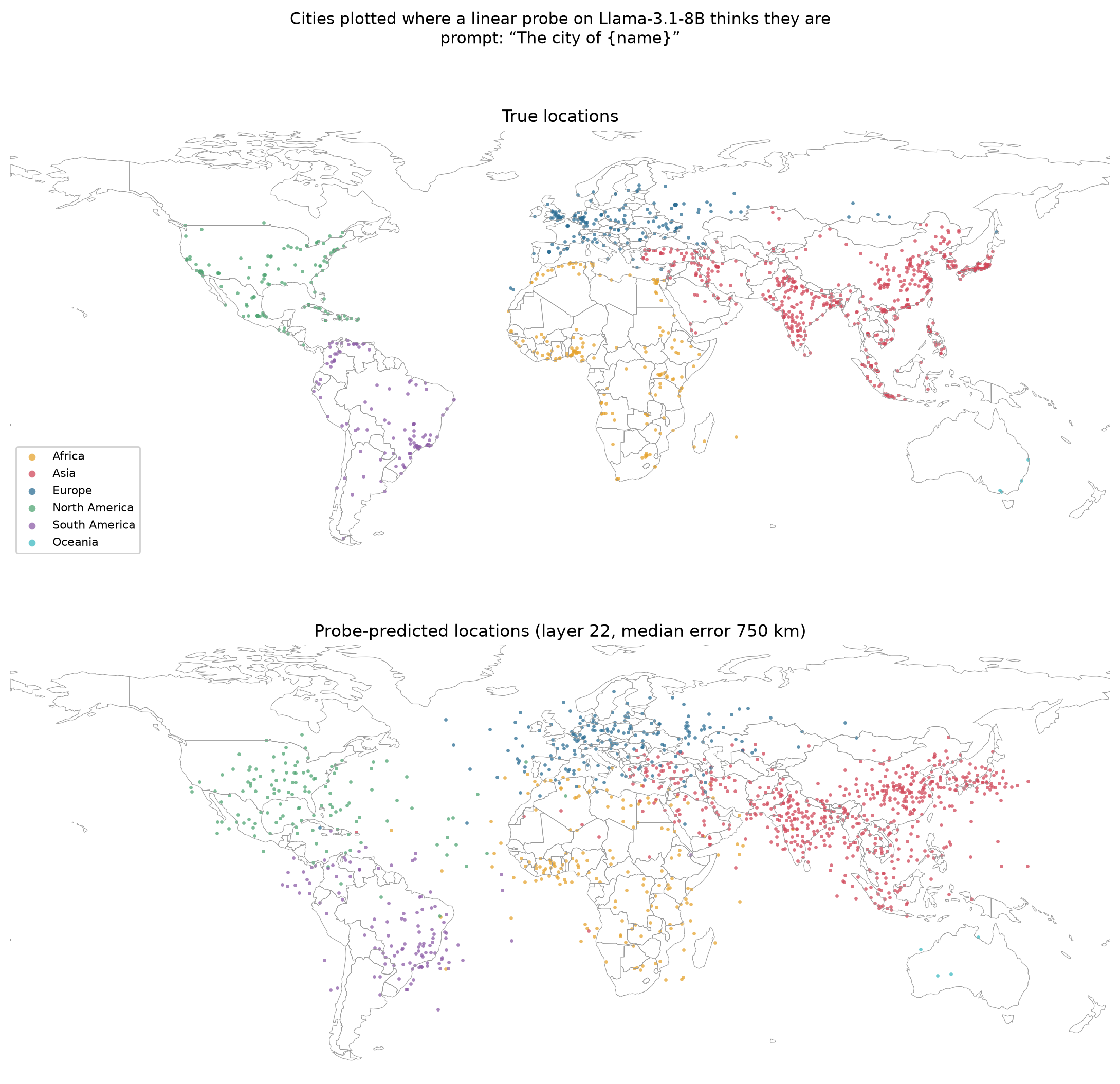
The city of {name},
layer 22. The probe was trained on disjoint cities.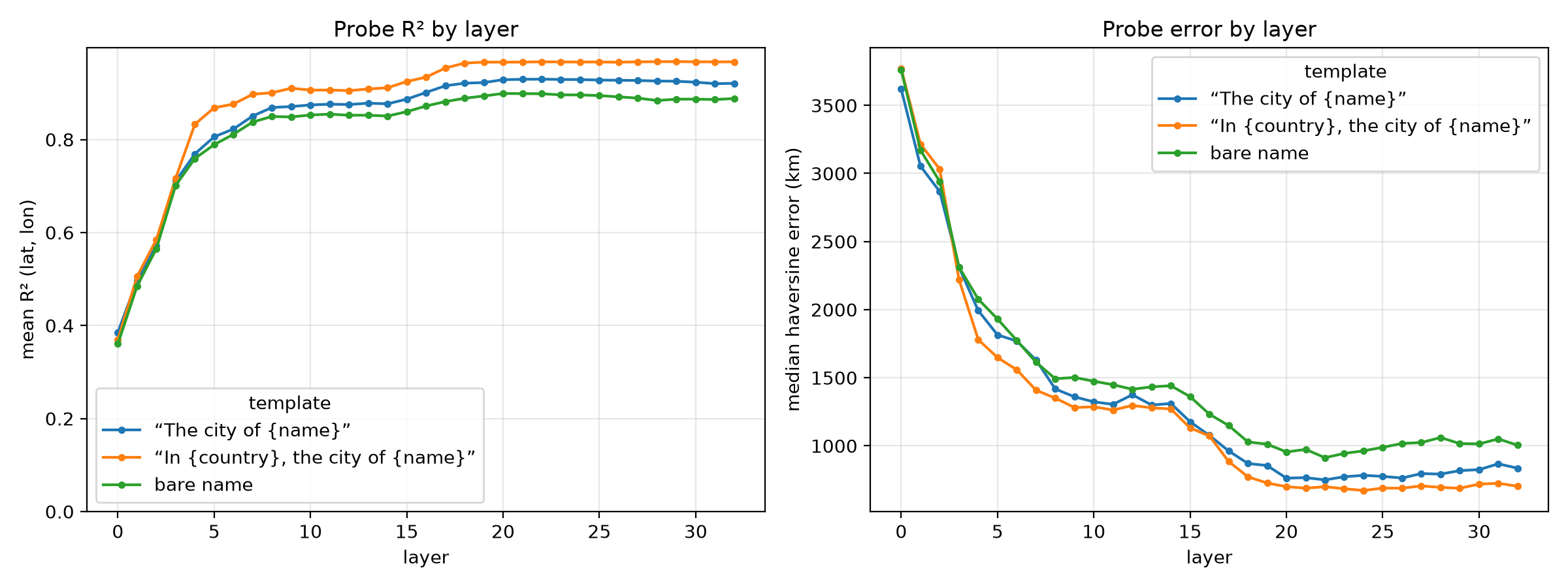
Looking at the layer sweep in Figure 3, there are two things I want to highlight. First, decodability is pretty low right at the embedding layer, but it goes up very quickly across layers 0 to 8 before plateauing near layer 20. This matches what Gurnee & Tegmark (2023) found regarding spatial features. Their theory is that this early-layer activity represents “entity resolution”. In other words, if a city name is broken into multiple text tokens, the network first has to stitch those together into a single, recognisable concept. Only after the model understands what the entity is can the deeper layers start adding semantic context, or in this case a sense of the geographical coordinates. The second observation is that we can also see how the model integrates context just by looking at the differences in the linear probes between templates. Just by conditioning on the country before the name, the \(R^2\) rises from 0.90 to 0.97, and the optimal layer is pushed later into the network (from 22 to 29). Essentially, the bare-name probe shows us what the model knows about the string by itself, whereas the country-conditioned probe gives a glimpse into how the network synthesises that name with its surrounding context.
City-Scale Granularity
Now that we have a decent read on the world-scale picture, let’s check whether this structure still exists as we zoom in. We already saw that country identity alone explains a lot of the world-scale variance, so a stricter test is whether position can be reliably decoded within a single city, where country gives you zero extra information.
To do this I used 1,087 named places inside Greater London (these include neighbourhoods,
districts, and villages) and probed with the template {name}, London, evaluated
with 5-fold cross-validation. For a baseline I used a constant predictor at the dataset
centroid, which gets a median error of 12.1 km. Against that, the probe does a lot better:
median error of 4.4 km (\(R^2 \approx 0.6\)).
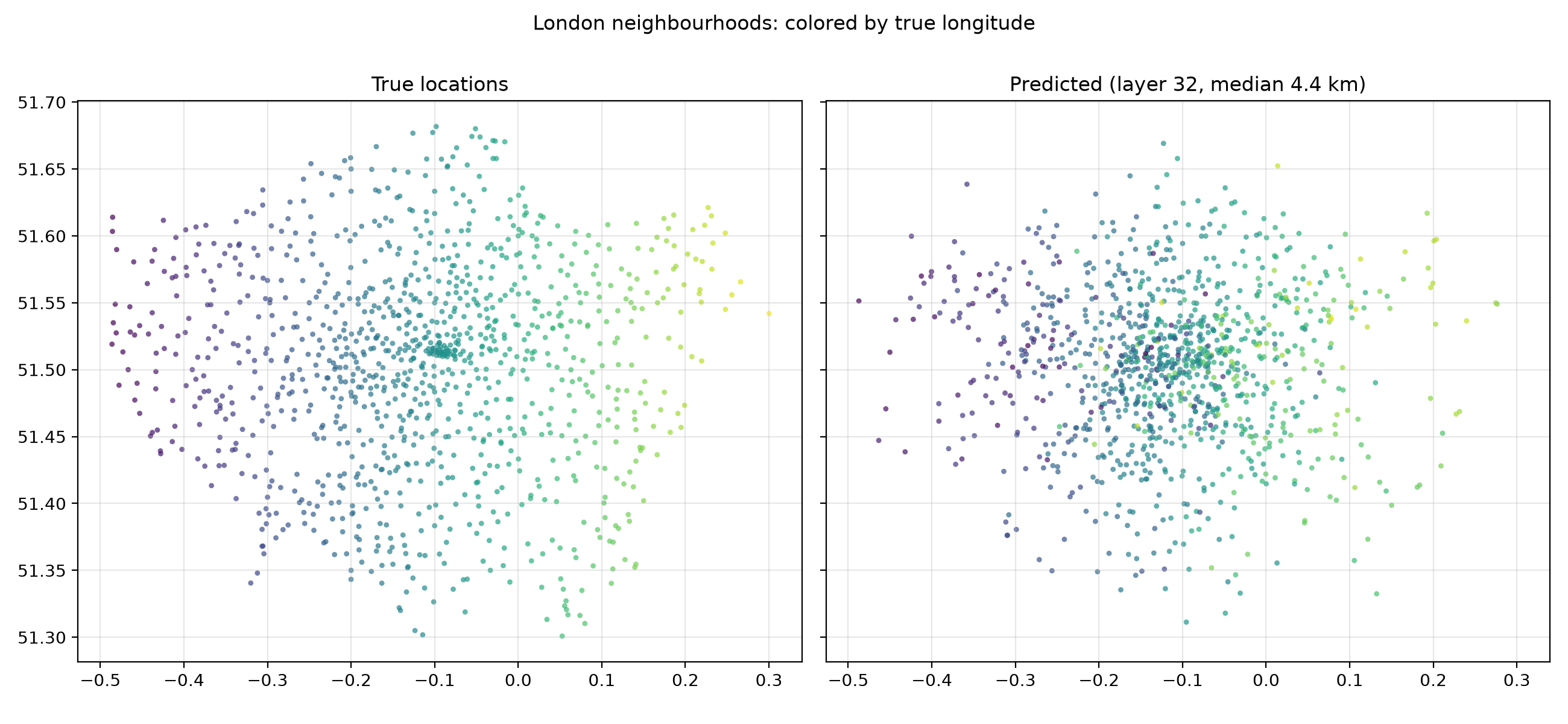
De Sabbata et al. (2025) also looked at spatial structure in LLM activations below country scale and found spatially correlated neurons across their geographical corpus (UK, Italy, and four US states). Testing this a different way, linear readout rather than neuron correlation, I find the same thing: spatial structure persists roughly two orders of magnitude below the scale Gurnee & Tegmark (2023) tested.
London is obviously a special case, since few places on Earth are documented this thoroughly, so let’s ask the same question of every country at once: after subtracting each country’s centroid, do the probe’s within-country deviations still track the true coordinates?
Turns out yes. Across all cities under the country-conditioned template, predicted and true deviations correlate at 0.35 (east–west) and 0.57 (north–south). That said, the probe only actually beats the country-centroid lookup in 6 of the 41 countries with at least 30 cities: Brazil, Canada, China, India, Russia, and the United States. So sub-country structure looks like it’s present pretty much everywhere, but whether a linear probe can out-predict a simple lookup table comes down to a country’s physical size relative to the probe’s noise floor: bigger countries give the probe more geographic variance to explain relative to its error, so it performs better there.
One interesting finding here is that the layer profile looks different from the world-scale case. Instead of saturating around layer 20, the London probe kept improving monotonically all the way to layer 32, the final one. I don’t have a solid intuition for why, but my best guess is that sub-city entities are rare enough that the model needs more layers of context integration to resolve them.
Error Structure
So far we have been able to confirm the finding reported by Gurnee & Tegmark (2023), and show that it extends to more granular spatial extents as well. But what exactly drives the error in predictions?
I looked at which places the probe gets wrong, and characterised the errors. To do this I gave every city an out-of-fold prediction via 5-fold cross-validation at the best layer, then checked if the per-city haversine error is random or if it correlates with things like region, population, or language. For region, I grouped cities by continent and compared median errors between groups; for population, I computed the correlation between a city’s population and its error; and lastly, for language, I looked into countries where English is the primary language vs not and compared their medians.
The table below shows continents sorted from best to worst median error.
| Continent | Median error (km) | 95% CI | n |
|---|---|---|---|
| Europe | 668 | [636, 704] | 948 |
| Asia | 688 | [662, 715] | 2,956 |
| Africa | 821 | [776, 885] | 830 |
| South America | 904 | [840, 974] | 631 |
| North America | 1,230 | [1,146, 1,341] | 651 |
| Oceania | 3,605 | [2,497, 5,591] | 32 |
The CIs are bootstrap intervals on the median.
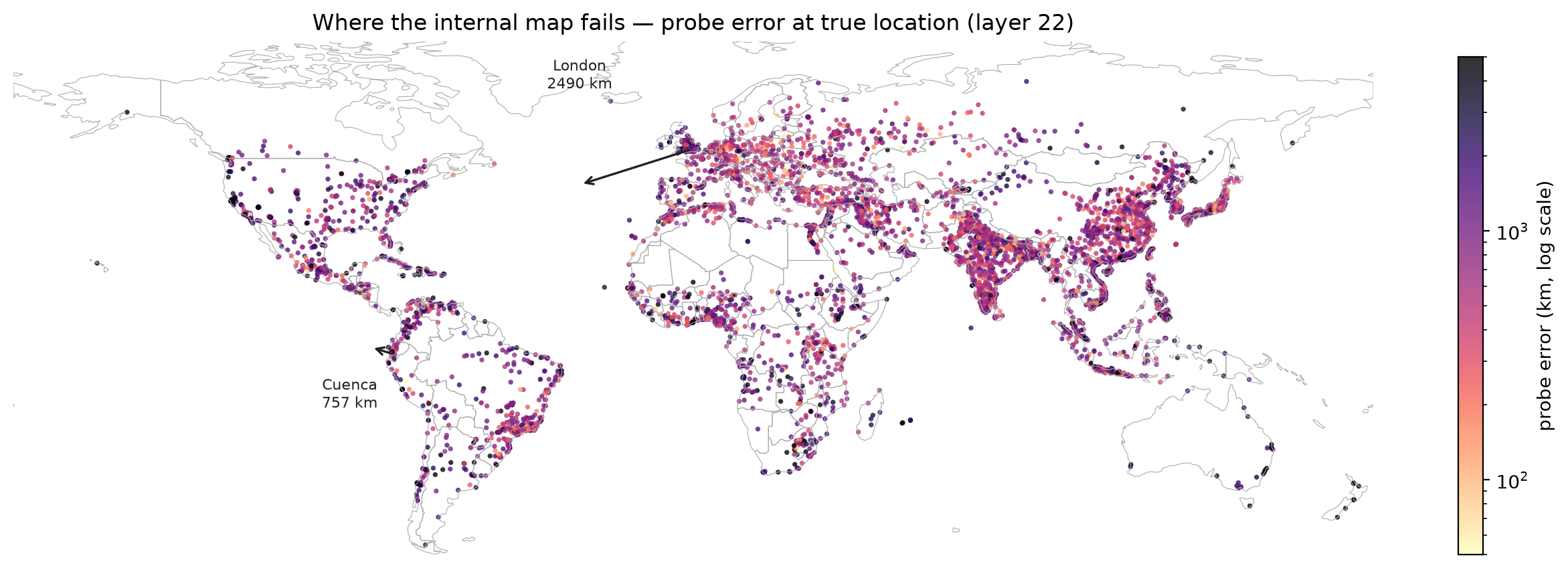
The city of
{name}, layer 22. Arrows show the displacement of two
example predictions: London (2,490 km) and Cuenca
(757 km).This continent-level ordering is at least partly consistent with the training-data coverage hypothesis: Africa’s median error is 23% higher than Europe’s, and South America’s is 35% higher. But the other coverage proxies tell a different story:
- Population. Probe error is basically uncorrelated with city population (Spearman \(\rho = -0.05\)). If coverage were the driver and assuming more populous cities are mentioned more frequently in the training corpus, we would expect the error to be lower.
- Language. Cities in countries where English is the primary language actually have slightly higher median error than the rest (780 km vs 751 km), the opposite of what the coverage hypothesis predicts.
- North America. The continent with the densest English-language coverage ranks second-worst overall.
Individual cities show the same results. Conditioned on country, the probe places Cuenca within 109 km and Quito within 192 km, while London, despite being one of the best-documented places in the dataset by any coverage measure, ends up placed 1,132 km away, out over the Atlantic; from the bare name alone, London’s error is 2,490 km (Fig. 5).
Name Ambiguity as a Source of Error
So, what does predict error? Turns out a good predictor is name ambiguity! In other words, how many distinct places share a city’s name. Take London: besides being the capital of the UK, it also names London, Ontario, and a handful of smaller settlements (London, Kentucky; London, Ohio). So every occurrence of the token in training text refers to a distribution over referents.
My hypothesis is that if the residual-stream representation of an ambiguous name is roughly a frequency-weighted mixture of its referents’ representations, a linear readout of coordinates should land somewhere between them. At least for London, that would explain it ending up in the North Atlantic with a linear probe (Fig. 6).

To test this beyond a couple of examples, I gave every city a namesake count: the number of GeoNames places with population above 15k that share its exact name. The correlation with probe error is weak in variance terms (\(\rho = 0.175\), only about 3% of rank variance) but large as a median shift: 734 km [715, 749] for unique names versus 1,278 km [1,156, 1,465] for shared names. North American toponyms reuse European ones at a high rate: for example, Birmingham, Manchester, Paris, and London all recur across the US and Canada. So namesake interference is concentrated there, and English-speaking countries hold most of the reused names. That points in the same direction as the result above.
But these are all univariate comparisons, and there are two possible explanations that are confounded. The first is the name ambiguity already mentioned, but there is a second possibility which is distance to the global centroid. Since ridge regression penalises large weights by construction, all predictions are pulled toward the mean of the training targets. So imagine the probe has perfectly good information about Vancouver: the ridge probe will still nudge its prediction some fraction of the way toward the Red Sea. For a city near the centroid, that nudge barely matters, but for a city that’s far away, that same proportional nudge generates large errors. To disentangle the effects, I regressed log error jointly on namesake count, distance from the training centroid, population, and continent; and since the shrinkage artifact doesn’t have to be linear in distance, I also repeated the distance control with decile dummies.
This is what I found: First, shrinkage induced by the linear probe explains a good part of the mean error differences between continents, and a flexible (non-linear) distance control explains even more of it than a simple linear control would: under that stricter control, North America (×1.14) and South America (×1.00) drop to non-significance, so their errors can be mostly explained by distance to the training centroid and name ambiguity. Africa (×1.34) and Oceania (×3.72) remain significant relative to Europe even under this control, so shrinkage and name ambiguity do not fully account for their errors. Second, namesake count turns out to be the single biggest predictor: ×1.53 error per doubling, with a partial \(\Delta R^2\) of 0.031, compared to 0.027 for the continent block and 0.006 for centroid distance. And it’s not just an artifact of the crude count either: an entropy-weighted ambiguity measure over namesake population shares gives the same rank correlation. Also, since deduplication keeps only the most populous holder of each name, every shared-name city here is the dominant referent, which is the case where ambiguity should have the least impact, so ×1.53 is really a lower bound.
Even after all these controls, Africa still carries a chunk of unexplained error, which kept hinting to me that there is a training-coverage issue: less text about African cities, worse coordinates. I don’t have a direct measure of “how much text mentions this place,” but I tried a couple of proxies. I pulled English Wikipedia articles for each city (matched through GeoNames link records, 4,924 of 6,048 cities); article length turns out to have essentially zero correlation with probe error (\(\rho = 0.005\)), and it’s the same story for the number of languages with a recorded name for the place (\(\rho = -0.014\)). Cities with no English article at all are only 8% worse than the rest, and adding this into the joint model only moves the Africa coefficient from ×1.39 to ×1.36. So documentation, at least as Wikipedia measures it, doesn’t seem to be impacting error. This also fits the population null from earlier. For now I’ll leave this unexplained, with OSM coverage as one future candidate to look at.
One more thing backs up the mixture interpretation: Context resolves the mixture. Under the country-conditioned template, the shared-name penalty shrinks quite a bit (median 928 km vs 686 km for unique names), and the namesake correlation drops from 0.175 to 0.111. So the model clearly can pick out the intended referent with the added context, even if not perfectly.
There’s a connection here to superposition (Elhage et al., 2022), which usually describes unrelated abstract features sharing the same directions in activation space. Here the interfering items are just different referents of the same token, and the interference is measurable in actual kilometres, which I think is a nice way to see it concretely.
To test this directly, I took 40 ambiguous names with referents spread across two to four
countries; extracted the bare-name activation and each referent’s country-conditioned
activation at the same layer; estimated the systematic offset between the two templates from
40 unique-name controls; and solved for the convex combination of referent activations that
comes closest to the bare activation. The true referents reduce the reconstruction residual by a
median of 9.4%, compared to just 2.3% for random cities’ activations and
2.8% for a matched null (same-country, similar-population distractor
cities); the true referents beat that matched null for 82%
of names. So the traces in the bare representation really are specific to
the actual referents, not just some generic sense of place-ness.
Interestingly, the recovered weights track textual prominence rather than
population: bare Valencia loads mostly on Valencia, Spain, even though
Valencia, Venezuela is actually the more populous city, and London
decomposes as roughly 0.65 on the UK capital and 0.35 on London, Ontario.
Read through a probe trained with these names held out, bare London
lands 21% of the way toward Ontario. But across all 35 two-referent
names, the median displacement is only 5% of the segment, and only half
the predictions even fall strictly between the referents. So the mixture
effect exists, but is usually pretty small.
Closing
So, a model trained only on next-token prediction over text ends up (approximately) linearly encoding coordinate systems that cover at least two orders of magnitude of spatial scale: a median error around 700 km for world cities and 4.4 km within London, both readable by ridge regression from a single activation vector. What makes the error structure interesting is that precision turns out to be nearly indifferent to how much text describes a place: population, article length, language breadth, even having an English Wikipedia article at all, don’t seem to matter much. What does degrade the map is ambiguity in the name, which pulls predictions toward rival referents, mildly for the typical name and severely in the tail, in a way that context can only partly correct.
References
- Alain, G. & Bengio, Y. (2016). Understanding intermediate layers using linear classifier probes. arXiv:1610.01644.
- Belinkov, Y. (2022). Probing classifiers: promises, shortcomings, and advances. Computational Linguistics, 48(1). arXiv:2102.12452.
- De Sabbata, S., Mizzaro, S. & Roitero, K. (2025). Geospatial mechanistic interpretability of large language models. arXiv:2505.03368; chapter in Janowicz, K. et al. (eds.), Geography According to ChatGPT, IOS Press, forthcoming.
- Elhage, N. et al. (2022). Toy models of superposition. Transformer Circuits Thread.
- Gurnee, W. & Tegmark, M. (2023). Language models represent space and time. arXiv:2310.02207.
- Hewitt, J. & Liang, P. (2019). Designing and interpreting probes with control tasks. Proceedings of EMNLP. arXiv:1909.03368.
- Liétard, B., Abdou, M. & Søgaard, A. (2021). Do language models know the way to Rome? arXiv:2109.07971. Proceedings of BlackboxNLP.
- GeoNames geographical database, geonames.org (CC BY 4.0).
total runtime is roughly one hour on an RTX 5080 laptop GPU (16 GB), of which activation extraction for 3 × 6,113 prompts takes about 15 minutes.